The function y(x) is represented by a series of tabulated values, pairs of x and y(x), plus a method for interpolating between input values. The pairs are ordered by increasing values of x. There will be NP pairs given. The complete region over which x is defined is broken up into NR interpolation ranges. An interpolation range is defined as a range of the indendent variable x in which a specified interpolation scheme can be use; i.e., the same scheme gives interpolated values of y(x) for any value of x within this range. The definitions of the quantities in the interpolation table follow:

Parameter Meaning NP Number of pairs x,y given NR Number of interpolation ranges given INT(m) interpolation scheme used in the mth range NBT(m) pair index separating the mth and (m+1)th ranges

The allowed interpolation schemes are

INT Meaning 1 y is constant in x (constant, histogram) 2 y is linear in x (linear-linear) 3 y is linear in ln(x) (linear-log) 4 ln(y) is linear in x (log-linear) 5 ln(y) is linear in ln(x) (log-log) 6 y obeys a Gamow charged-particle penetrability law

Interpolation code INT=1 (constant) implies that the function is constant and equal to the value given at the lower limit of the interval.

Note that where a function is discontinuous (for example, when resonance parameters are used to specify the cross section in one range), the value of x is repeated and two different y values are given to make a discontinuity.

Examples of Interpolation Tables

The most common interpolation table in the ENDF/B files simply specifies that linear-linear interpolation is used throughout the range of x.

      NR=1
      NP=10

      10    2

      NR=3
      NP=10

      2    2    6    5    10    1

Charged-Particle Cross Sections

A special one-dimensional interpolation law, INT=6, is defined for charged-particle cross sections. It is based on the limiting forms of the Coulomb penetrabilities for exothermic reactions at low energies and for endothermic reactions near the threshold. This scheme gives a concave upward energy dependence near the threshold that is quite different from the behavior of the neutron cross sections. At higher energies, non-exponential behavior will normally begin to appear, and linear-linear interpolation is more suitable. The formulas for INT=6 follow:

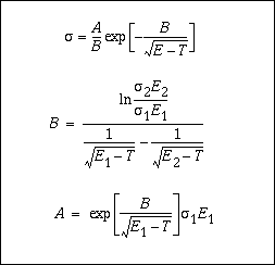
where E₁,σ₁ and E₂,σ₂ are two consecutive points in the cross-section tabulation. In these formulas, T=0 for exothermic reactions (Q>0). For endothermic reactions, T is the kinematic threshold.